As many of you know, I’m taking, for career change and self improvement, a certified curriculum offered by Columbia University and Microsoft and edX.org, on Data Science. With this, I hope to be able to change careers from Systems Engineering (which I love, but had become limiting) to a job in Data Analysis/Data Science, which will take me out of the Operations/Data/Server Center and into a cushy not-on-call job in a loving data haven.
One of the things they insist you learn in Data Science is statistics. About which I have conflicted feelings (statistics, not having to learn it for Data Science). But it’s been good for me. If I’m going to be snooty about something, I should probably understand it/have experienced it/tried it out. (Thus why I spent a year in a Bible Study group. And why I volunteer for service jobs. And why I try not to have Opinions about that which I know nothing.)
Statistics (my first of 3 courses on it, mind you), has taught me a lot so far. The reason that while I was definitely going to pass that class, I still took a couple of weeks to really try to understand part of it that I was stuck on was again, not wanting to be snooty about something I didn’t understand. And that thing was Bayesian Conditional Probability. It’s an interesting field in dependent probability. Using the methodology, you can meaningfully assess probability and risk of conditional and interdependent things happening. It’s the Monty Hall problem, and also why a lot of us can’t help but figure (wrongly, it turns out, or misguidedly, at least) that since the Lotto hasn’t yet been won, it’s just GOTTA BE this week. But more practically, it’s also why you shouldn’t let one test result convince you that you have medical condition X. This was a result I never knew about before taking this class, and as we get older, it becomes more and more important (more tests, more test results, more medical decisions).
I’m writing about it here because you probably don’t know about it either, and I hope that it will help you avoid feeling pressed, if you get an alarming medical test result sometime. The reason we don’t know about it is that few schools teach conditional probability in basic education, and because it can be hard to figure out when one probability is dependent upon another.
We end up learning that probabilities are (and they sometimes are) independent. This is a good lesson for playing the Lotto, but not a great lesson for other probabilities and risks, like lab tests and playing games with Monty Hall.
Incidentally, another explanation (that I’m basing this on) of conditional probability that I quite like is in The Cartoon Guide to Statistics, by Larry Gonick and Woollcott Smith, Chapter 3, p 27 – 52. If, as I did, you get stuck on a single explanation, do go check it out. It’s quite well done.
Anyhow, suppose a disease’s incidence in the general population is 1 in 1000. And suppose your doctor convinces you to take a test for it and you test positive. The test is pretty good but not certain. The probability of a positive test, given infection, is 99%, and the probability of a false positive (getting a positive test when you don’t have the infection) is 2%. Seems reasonable to worry, right?
So here’s the setup. Let’s observe that there are two dependent, conditional events here:
- Event A: Patient has the disease
- Event B: Patient tests positive with the test
Here is the info we have about the disease, the test, and the testing space.
- Probability of having the disease, P(A) = 0.001
- Probability of a positive test, given infection, P(B|A) = 0.99
- Probability of a false positive, given no infection, P(B|NOT A) = 0.02
And our ultimate question:
- Probability of having the disease, given a positive test, P(A|B) = ???
Now, a table!
Here is the problem space:
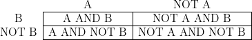
And here are the probabilities for each event:
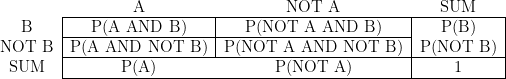
In Conditional Probabilities, it’s often easier to compute the reverse of some probability and subtract it from one. ALSO, it’s easy to miss a possible event (or permutation or possibility) in the space, so it’s good to use a table or other device so you don’t miss anything. For any particular event space, the total probabilities should add up to 1, because when you do something, there ought to be an observable result so statistics can work. It’s a little metaphysical, but there is a certainty that something will happen, so that’s 100% or 1. 0% is 0, and you can’t have negative probabilities, ever.
Anyhow, to return to our problem of finding out P(A|B), let’s do the following:
Compute:
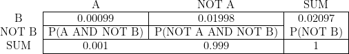
P(A AND B) = P(B|A)P(A)
We know these probabilities on the right, so it’s:
(0.99)(0.001) = 0.00099
Also compute:
P(NOT A AND B) = P(B|NOT A)P(NOT A)
Which we also know:
(0.02)(0.999) = 0.01998
(Those zeroes really add/multiply up!)
So now the table looks like:
Find the remaining probabilities by subtraction:

From which we can calculate:
P(A|B)


= 0.0472
So. Despite the high accuracy of the test, there’s less than 5% chance that, given a positive test result that you actually have the infection. To me, this result is totally weird and quite nonintuitive given how awesome the test’s probabilities seemed. But the math is there, and it makes sense. What are the indications for you and your doctor should you encounter a positive test? Do more tests with different characteristics. Layer this result with others to be sure.
And don’t let yourself be ruled by statistics. Especially if you don’t really understand them. Learn about them or learn from others about when to take statistics at face value and when to question them and look deeper. The answer is: almost always, look deeper.
(Also note: Because it’s all math and deeply dependent on starting conditions, be aware that this particular result is highly dependent on the initial conditions. Remember that for any test or disease, the incidence changes, the rates of positives and negatives change, and so it is absolutely wrong to say all tests go this way. You’d need to calculate for each individual disease/test if you were looking for a general indicator of effectiveness. This is just an example, but still quite surprising, I think.)